
If you are dealing with data duplication in Microsoft Excel, then this guide aims to show you effective ways to tackle this problem. Make sure that you remove the blank spaces in the data before continuing with these methods.
Highlighting the Duplicated Data:
First, you will need to track the data that has been duplicated. In order to do that, follow these steps:
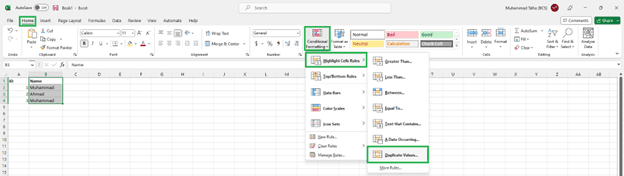
- Select all the data that you want to check against. Click on ‘Home’ tab located at the top.
- Click on ‘Conditional Formatting’, then on ‘Highlight Cell Rules’. Now click on ‘Duplicate Values’.
- Make sure that the drop-down menu on the left is selected to ‘Duplicate’. Then choose the color to highlight them from the drop-down menu on the right.
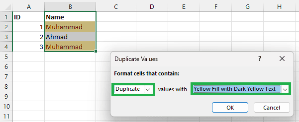
- This will highlight the duplicated values. Now it is up to you to decide what you want to do with the data.
Removing Duplicates:
You can use Excel’s built-in feature to remove the duplicated data. Follow the steps mentioned below:
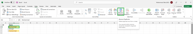
- Click on a cell with data. Select the ‘Data’ tab from the top. Then click on ‘Remove Duplicates’ option.
- Select the columns in which you want the duplicated data to be searched. Click on OK.
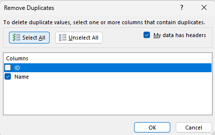
- The duplicated data will be removed.
Using the Unique Function:
If you use the ‘UNIQUE’ function in Excel, you can gain the data with no duplication. However, it doesn’t overwrite the existing data, rather it returns new data. Here’s how you can do it:
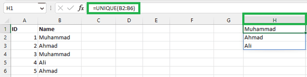
- Select an empty column in Excel in which you want the data to be displayed. Write the UNIQUE function in the formula bar at the top.
- Type it like this:
=UNIQUE(B2:B6) - In place of ‘B2’ and ‘B6’, you have to write the cell range for your data. This will search the input cell range and then return the unique values from that range.
These were some effective ways to deal with data duplication in MS Excel. Hopefully, this guide proves useful to you.